import shinybroker as sb
from shiny import Inputs, Outputs, Session, reactive


# Declare a server function...
#   ...just like you would when making an ordinary Shiny app.
def step_1_server(
        input: Inputs, output: Outputs, session: Session, ib_socket, sb_rvs
):

    @reactive.effect
    @reactive.event(sb_rvs['connection_info'])
    def make_historical_data_queries():

        # Fetch the hourly trade data for AAPL for the past 3 days.
        sb.start_historical_data_subscription(
            historical_data=sb_rvs['historical_data'],
            hd_socket=ib_socket,
            contract=sb.Contract({
                'symbol': "AAPL",
                'secType': "STK",
                'exchange': "SMART",
                'currency': "USD",
            }),
            durationStr="3 D",
            barSizeSetting="1 hour"
        )

        # Do the same, but for the S&P 500 Index
        sb.start_historical_data_subscription(
            historical_data=sb_rvs['historical_data'],
            hd_socket=ib_socket,
            contract=sb.Contract({
                'symbol': 'SPX',
                'secType': 'IND',
                'currency': 'USD',
                'exchange': 'CBOE'
            }),
            durationStr="3 D",
            barSizeSetting="1 hour"
        )


# create an app object using your server function
# Adjust your connection parameters if not using the default TWS paper trader,
#   or if you want a different client id, etc.
app = sb.sb_app(
    server_fn=step_1_server,
    host='127.0.0.1',
    port=7497,
    client_id=10799,
    verbose=True
)

# run the app.
app.run()Query and Display Market Data
So you’ve installed Shinybroker and gotten the hello world example to work. Congrats! Now it’s time to actually build an app that uses some of the features.
This example will introduce you, in steps, to using ShinyBroker to write an app that will calculate beta between two assets, display that information, and use it to trade. Each step below adds a layer of functionality to the app. You can use this example to learn how to:
- access & use the ShinyBroker reactive variables in
sb_rvs - implement some initial setup logic to fetch data from IBKR
- process your data and display it
Coming Soon: live updating data, dynamic contract entry, positions, order placement, and finally– a video walkthrough of all this :)
Step 1: sb_rvs and setup logic
We’re interested in calculating beta between two assets, so first we’re going to need to pull price data from IBKR in order to make the calculation. We can accomplish this task by writing a server function that sends the data request query to the IBKR data farms.
The Design Pattern
The server function, appropriately named step_1_server, contains within it a single function named make_historical_data_queries(), which is decorated with reactive effect and reactive event.
Why sb_rvs['connection_info'] is a good trigger for startup logic
Because it is a reactive event that takes sb_rvs['connection_info'], as a dependency, the code in make_historical_data_queries() will only run when the reactive variable sb_rvs['connection_info'] is updated. However, sb_rvs['connection_info'] is only updated once during the running lifetime of a ShinyBroker session. Since the update takes place right after a socket connection has been made to the client (e.g., TWS), you, the trader, can be sure that if sb_rvs['connection_info'] has been successfully set, then the socket connection is connected and ready for use. Therefore, sb_rvs[‘connection_info’] makes a good choice for a trigger for logic that you want to run only once at the beginning of a user session in your app.
The Setup Function: make_historical_data_queries
Once triggered, make_historical_data_queries makes two calls to start_historical_data_subscription, a function provided by the ShinyBroker library. Even though in this case we’re performing a static, one-time data query, the word “subscription” appears in the function’s name because it can be called by setting the keepUpToDate parameter to True. Doing so results in the historical data being kept up-to-date with live market data as it becomes available, and we’ll do exactly this in a later step.
For now, you should understand four things about start_historical_data_subscription:
- The data it fetches is written to the reactive variable named ‘historical_data’. Because this is a native ShinyBroker reactive variable, you can always access it in your code with
sb_rvs['historical_data'] sb_rvs['historical_data']()is a dictionary that contains the data retrieved by each query. That dictionary is keyed by the integer-valuedsubscription_idyou pass to it. If you don’t pass a subscription id, as in the code below, then ShinyBroker will just find the maximum subscription id already used in a historical data query for that session, add1to that, and treat the result as thesubscription_id, beginning with1if no previous subscriptions are found for the current session.- You must define the
contractfor which you want data using theContractconstructor, which is provided by the ShinyBroker package. - As currently written, you must tell
start_historical_data_subscriptionwhich IBKR connection socket you want it to use by defining thehd_socketparameter. In the code below, the defaultib_socketprovided by the ShinyBroker app is used. This choice was made by the ShinyBroker author in order to allow advanced users to work with more than one socket connection within their apps. Most users of ShinyBroker won’t need that functionality and can just keep passingib_socketas the socket parameter in their apps without having to think too much about it.
Run the code below
Run the code!
- View your Shiny app in a browser by clicking the hyperlink that prints in your Python console
- Within the app, navigate to the Market Data panel
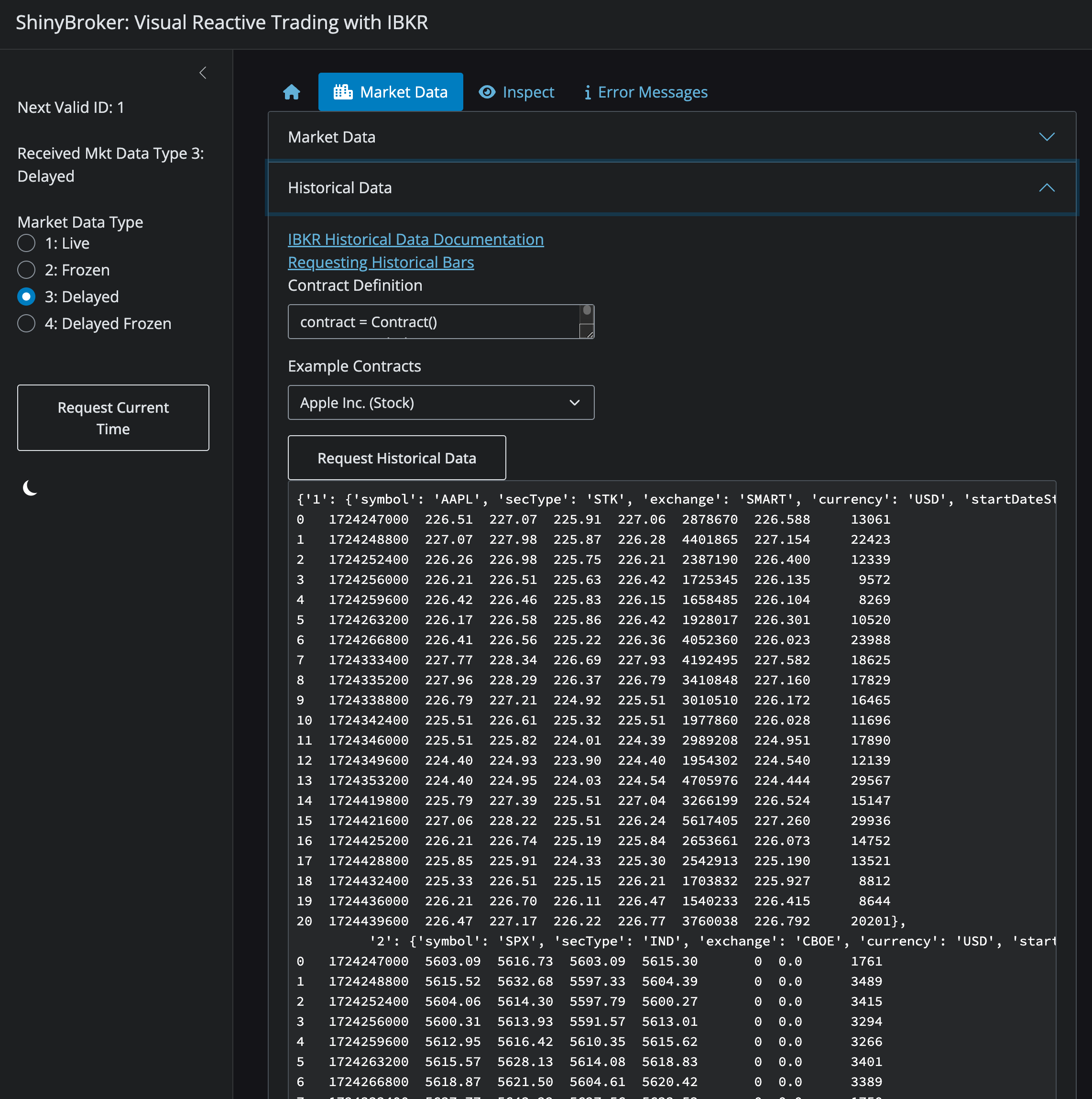
- Open the “Historical Data” accordion panel… …and you should see an output of the historical data fetched by your query that looks something like the below:
 Once you’ve successfully accomplished that, you can move on to the next step!
Code:
Step 2: Calculations and ui
In this step we’ll add the calculations of alpha and beta, including the observed historical returns over the time period, plus the necessary pieces of UI to display the calculated information. We’ll be using some additional Python libraries to accomplish this task:
- faicons
- plotly
- sklearn, which is available after installing scikit-learn
…so make sure those libraries are installed.
The UI
The code below follows the same general design pattern of Step 1, but adds in a ui object named step_2_ui. This object contains within it the HTML structure that sb_app() will place in the Home tab of the rendered app. Reference documentation for for these and other webpage-generating ui objects available within Shiny can be found on Shiny’s documentation page.
Examine the definition of step_2_ui in the code below. You will notice that it contains the four new ui features that have been added in this step:
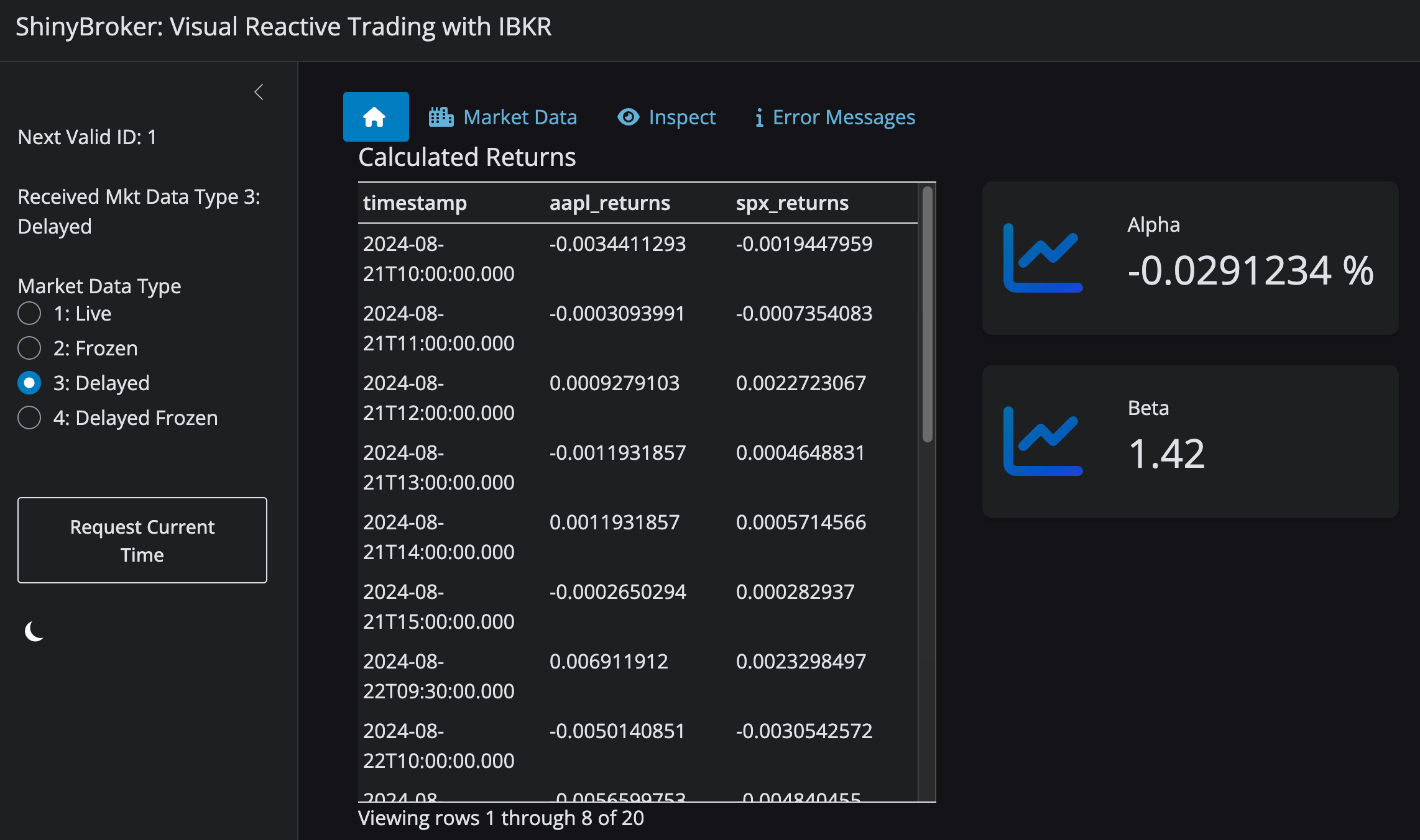
- An HTML level 5 title tag which reads ‘Calculated Returns’
- A dataframe output that displays the returns calculated for the two assets
- An info box for calculated alpha value
- An info box for calculated beta value
Any valid Shiny ui object passed to sb_app() will be rendered in the Home tab.
The Server Function
In order to populate the new ui objects with data, we need to add logic to the server function.
The calculate_log_returns() Function
The reactive calculation that operates on the retrieved historical data is named calculate_log_returns(). The function operates as follows:
First, it looks at the data stored in sb_rvs['historical_data'] and assigns it to a new variable hd for the analysis. If hd doesn’t contain TWO entries – one for AAPL and one for SPX – then a KeyError exception gets raised when attempting to declare aapl_rtns and spx_rtns. In that case, calculate_log_returns() exits early and returns None because we need data
Calculation proceeds otherwise. The period-over-period log returns are calculated for each asset and stored in two dataframes named asset_1 and asset_2 alongside a column named timestamp that contains the date & time at which each return was observed.
Note that in order to make this datetime conversion easier, the calls to start_historical_data_subscription were made with the formatDate argument set to 2. IBKR’s documentation for historical data requests tells us that datetimes received with this choice of parameter will be in Unix Epoch Date format, which is nice and easy to handle in Python for datetime conversions.
Once dataframes for both asset_1 and asset_2 are calculated, they are merged together via an inner join on timestamp. The reason for doing so is because sometimes, one asset might be updated before the other one, meaning that it has one more measured return. By creating a new df using the merge on datetime, we ensure that our returns match up for an equal number of observations of both assets.
That merged dataframe is the return value of calculate_log_returns(). Therefore, when calculate_log_returns() is called within any other reactive function in the app, Shiny will ensure that the value returned always contains the most up-to-date calculation, even if the historical data changes.
A @render Function: log_returns_df()
In the Shiny world, to “render” means “to display the contents of variables as UI objects in an app”. Because it has the [dataframe render decorator] (https://shiny.posit.co/py/api/core/render.data_frame.html), Shiny knows to look for a UI object having the same ID as the name of the function and update that ui object with HTML that displays the returns in the dataframe calculated by calculate_log_returns(). If calculate_log_returns() returns None, then log_returns_df() exits early with a silent exception that does nothing.
To summarize: this simple function says the following to Shiny: “whenever the value of ’calculate_log_returns()` changes, render the output as html and insert it into the ui object named having the same name as this function (which in this case is”log_returns_df”)“. Therefore, the data in the datatable display in the UI will always be kept up to date with the historical data calculation.
Declaring alpha and beta as reactive variables
Next we define two new reactive variables– alpha and beta. Once they are set, follow-on code can call them to perform whatever calculations you like; for for example, you might have some specific trading logic you’d like to trigger if beta moves beyond a threshold that you set. We can calculate values for them by finding the y-intercept and slope of a linear regression fitted through the returns data with SPX on the x-axis as described below.
The update_alpha_beta() Function
update_alpha_beta() is a reactive effect function that uses sklearn to fit a basic linear regression model to the calculated returns, with the benchmark (SPX) on the X axis and the asset (AAPL) on the Y. Beta is defined as the slope of the regression, and alpha is the x-intercept. Each parameter thus obtained is set to its respective reactive variable.
Rendering the Value Box Text
Finally, the last two functions place text values in the value boxes for display to the user. They take in alpha and beta, perform some string manipulation, and put the result in the UI text object having the same name as the function definition. Because these UI objects were defined as the value parameter within the value box definition in step_2_ui, the value box’s contents gets updated for the user. The call to req is performed to require that the incoming variable is something other than an empty float.
Run & View the App
When you see something like the below when you run your app, you are successful! Move on to the next step when ready :) 
Code:
import numpy as np
import pandas as pd
import shinybroker as sb

from datetime import datetime
from faicons import icon_svg
from sklearn import linear_model
from shiny import Inputs, Outputs, Session, reactive, ui, req, render
from shiny.types import SilentException

step_2_ui = ui.page_fluid(
    ui.row(
        ui.h5('Calculated Returns'),
        ui.column(
            7,
            ui.output_data_frame('log_returns_df')
        ),
        ui.column(
            5,
            ui.value_box(
                title="Alpha",
                value=ui.output_ui('alpha_txt'),
                showcase=icon_svg('chart-line')
            ),
            ui.value_box(
                title="Beta",
                value=ui.output_ui('beta_txt'),
                showcase=icon_svg('chart-line')
            )
        )
    )
)


# Declare a server function...
#   ...just like you would when making an ordinary Shiny app.
def step_2_server(
        input: Inputs, output: Outputs, session: Session, ib_socket, sb_rvs
):

    @reactive.effect
    @reactive.event(sb_rvs['connection_info'])
    def make_historical_data_queries():

        # Fetch the hourly trade data for AAPL for the past 3 days.
        sb.start_historical_data_subscription(
            historical_data=sb_rvs['historical_data'],
            hd_socket=ib_socket,
            contract=sb.Contract({
                'symbol': "AAPL",
                'secType': "STK",
                'exchange': "SMART",
                'currency': "USD",
            }),
            durationStr="3 D",
            barSizeSetting="1 hour",
            formatDate=2
        )

        # Do the same, but for the S&P 500 Index
        sb.start_historical_data_subscription(
            historical_data=sb_rvs['historical_data'],
            hd_socket=ib_socket,
            contract=sb.Contract({
                'symbol': 'SPX',
                'secType': 'IND',
                'currency': 'USD',
                'exchange': 'CBOE'
            }),
            durationStr="3 D",
            barSizeSetting="1 hour",
            formatDate=2
        )

    @reactive.calc
    def calculate_log_returns():
        hd = sb_rvs['historical_data']()

        # Make sure that BOTH assets have been added to historical_data
        try:
            aapl_rtns = hd['1']['hst_dta']
            spx_rtns  = hd['2']['hst_dta']
        except KeyError:
            return None

        asset_1 = pd.DataFrame({
            'timestamp': [
                datetime.fromtimestamp(int(x)) for
                x in hd['1']['hst_dta'].loc[1:, 'timestamp']
            ],
            'aapl_returns': np.log(
                aapl_rtns.loc[1:, 'close'].reset_index(drop=True) /
                aapl_rtns.iloc[:-1]['close'].reset_index(drop=True)
            )
        })
        asset_2 = pd.DataFrame({
            'timestamp': [
                datetime.fromtimestamp(int(x)) for
                x in hd['2']['hst_dta'].loc[1:, 'timestamp']
            ],
            'spx_returns': np.log(
                spx_rtns.loc[1:, 'close'].reset_index(drop=True) /
                spx_rtns.iloc[:-1]['close'].reset_index(drop=True)
            )
        })
        return pd.merge(asset_1, asset_2, on='timestamp', how='inner')

    @render.data_frame
    def log_returns_df():
        if calculate_log_returns() is None:
            raise SilentException()
        return render.DataTable(calculate_log_returns())

    alpha = reactive.value(float())
    beta = reactive.value(float())

    @reactive.effect
    def update_alpha_beta():
        log_rtns = calculate_log_returns()

        if log_rtns is None:
            raise SilentException()

        regr = linear_model.LinearRegression()
        regr.fit(
            log_rtns.spx_returns.values.reshape(log_rtns.shape[0], 1),
            log_rtns.aapl_returns.values.reshape(log_rtns.shape[0], 1)
        )
        alpha.set(regr.intercept_[0])
        beta.set(regr.coef_[0][0])

    @render.text
    def alpha_txt():
        a = req(alpha())
        return f"{a * 100:.7f} %"

    @render.text
    def beta_txt():
        b = req(beta())
        return str(round(b, 3))


# create an app object using your server function
# Adjust your connection parameters if not using the default TWS paper trader,
#   or if you want a different client id, etc.
app = sb.sb_app(
    home_ui=step_2_ui,
    server_fn=step_2_server,
    host='127.0.0.1',
    port=7497,
    client_id=10799,
    verbose=True
)

# run the app.
app.run()
Step 3: Add a plot!
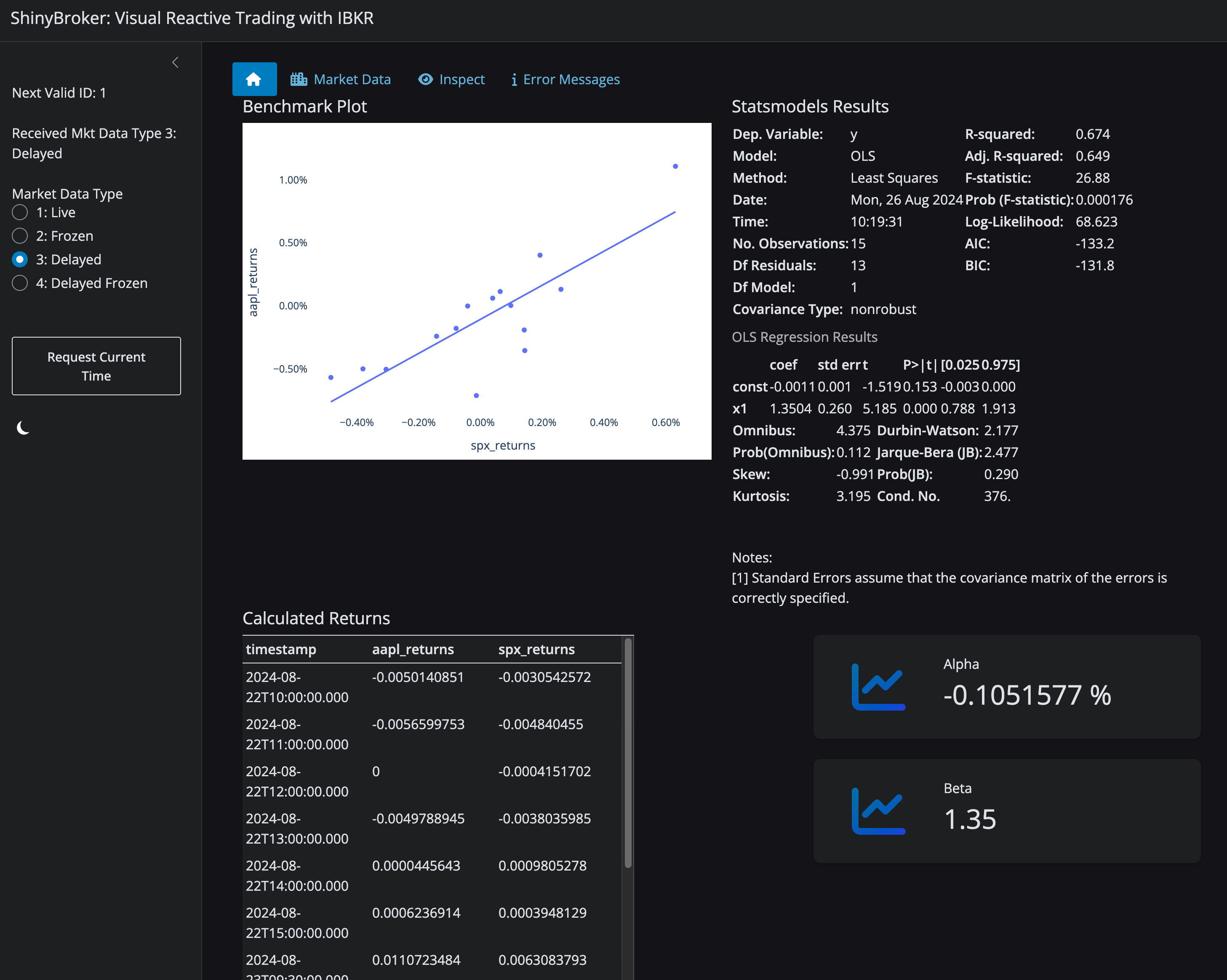
Every good app needs a plot. In the code below, we add a reactive calc for a plotly scatterplot object named fig within the server code. We also add two render functions. The first one renders the plot object display graphic. Since plotly includes a trendline feature using statsmodels, we make use of that feature by adding an ‘ols’ trendline. We also add a render function that selects and returns the summary property of the ols trendline and renders it as html next to the benchmark plot.
And of course, we add output elements for these new features in to the ui definition where the plot and table output for our alpha & beta calcs will be displayed in the top row of the *Home** section.
NOTE FOR MAC USERS and anyone else experiencing an ImportError saying something like “symbol not found in flat namespace ’_npy_cabs’“: There is a known bug between statsmodels and SciPy that causes a problem when you try to add trendlines to a Plotly chart in Python running in OSX. Until the bug is fixed, the workaround is to simply revert to numpy version 2. You can do that in one step with the shell command pip install --force-reinstall numpy==2.0.0.
Success means you can get your app to look like this: 
Code:
import numpy as np
import pandas as pd
import shinybroker as sb
import plotly.express as px

from datetime import datetime
from faicons import icon_svg
from sklearn import linear_model
from shiny import Inputs, Outputs, Session, reactive, ui, req, render
from shiny.types import SilentException
from shinywidgets import output_widget, render_plotly

step_3_ui = ui.page_fluid(
    ui.row(
        ui.column(
            6,
            ui.h5("Benchmark Plot"),
            output_widget("alphabeta_scatter")
        ),
        ui.column(
            6,
            ui.h5("Statsmodels Results"),
            ui.output_ui("alphabeta_trendline_summary")
        )
    ),
    ui.row(
        ui.h5('Calculated Returns'),
        ui.column(
            7,
            ui.output_data_frame('log_returns_df')
        ),
        ui.column(
            5,
            ui.value_box(
                title="Alpha",
                value=ui.output_ui('alpha_txt'),
                showcase=icon_svg('chart-line')
            ),
            ui.value_box(
                title="Beta",
                value=ui.output_ui('beta_txt'),
                showcase=icon_svg('chart-line')
            )
        )
    )
)

# Declare a server function...
#   ...just like you would when making an ordinary Shiny app.
def step_3_server(
        input: Inputs, output: Outputs, session: Session, ib_socket, sb_rvs
):

    @reactive.effect
    @reactive.event(sb_rvs['connection_info'])
    def make_historical_data_queries():

        # Fetch the hourly trade data for AAPL for the past 3 days.
        sb.start_historical_data_subscription(
            historical_data=sb_rvs['historical_data'],
            hd_socket=ib_socket,
            contract=sb.Contract({
                'symbol': "AAPL",
                'secType': "STK",
                'exchange': "SMART",
                'currency': "USD",
            }),
            durationStr="3 D",
            barSizeSetting="1 hour",
            formatDate=2
        )

        # Do the same, but for the S&P 500 Index
        sb.start_historical_data_subscription(
            historical_data=sb_rvs['historical_data'],
            hd_socket=ib_socket,
            contract=sb.Contract({
                'symbol': 'SPX',
                'secType': 'IND',
                'currency': 'USD',
                'exchange': 'CBOE'
            }),
            durationStr="3 D",
            barSizeSetting="1 hour",
            formatDate=2
        )

    @reactive.calc
    def calculate_log_returns():
        hd = sb_rvs['historical_data']()

        # Make sure that BOTH assets have been added to historical_data
        try:
            aapl_rtns = hd['1']['hst_dta']
            spx_rtns = hd['2']['hst_dta']
        except KeyError:
            return None

        asset_1 = pd.DataFrame({
            'timestamp': [
                datetime.fromtimestamp(int(x)) for
                x in hd['1']['hst_dta'].loc[1:, 'timestamp']
            ],
            'aapl_returns': np.log(
                aapl_rtns.loc[1:, 'close'].reset_index(drop=True) /
                aapl_rtns.iloc[:-1]['close'].reset_index(drop=True)
            )
        })
        asset_2 = pd.DataFrame({
            'timestamp': [
                datetime.fromtimestamp(int(x)) for
                x in hd['2']['hst_dta'].loc[1:, 'timestamp']
            ],
            'spx_returns': np.log(
                spx_rtns.loc[1:, 'close'].reset_index(drop=True) /
                spx_rtns.iloc[:-1]['close'].reset_index(drop=True)
            )
        })

        return pd.merge(asset_1, asset_2, on='timestamp', how='inner')

    @render.data_frame
    def log_returns_df():
        if calculate_log_returns() is None:
            raise SilentException()
        return render.DataTable(calculate_log_returns())

    alpha = reactive.value(float())
    beta = reactive.value(float())

    @reactive.effect
    def update_alpha_beta():
        log_rtns = calculate_log_returns()

        if log_rtns is None:
            raise SilentException()

        regr = linear_model.LinearRegression()
        regr.fit(
            log_rtns.spx_returns.values.reshape(log_rtns.shape[0], 1),
            log_rtns.aapl_returns.values.reshape(log_rtns.shape[0], 1)
        )
        alpha.set(regr.intercept_[0])
        beta.set(regr.coef_[0][0])

    @render.text
    def alpha_txt():
        a = req(alpha())
        return f"{a * 100:.7f} %"

    @render.text
    def beta_txt():
        b = req(beta())
        return str(round(b, 3))

    @reactive.calc
    def calculate_alphabeta_scatter():
        log_rtns = calculate_log_returns()

        if log_rtns is None:
            raise SilentException()

        fig = px.scatter(
            log_rtns,
            x='spx_returns',
            y='aapl_returns',
            trendline='ols'
        )
        fig.layout.xaxis.tickformat = ',.2%'
        fig.layout.yaxis.tickformat = ',.2%'
        fig.update_layout(plot_bgcolor='white')
        return fig

    @render_plotly
    def alphabeta_scatter():
        return calculate_alphabeta_scatter()

    @render.ui
    def alphabeta_trendline_summary():
        summy = px.get_trendline_results(
            calculate_alphabeta_scatter()
        ).px_fit_results.iloc[0].summary().as_html()
        return ui.HTML(summy)


# create an app object using your server function
# Adjust your connection parameters if not using the default TWS paper trader,
#   or if you want a different client id, etc.
app = sb.sb_app(
    home_ui=step_3_ui,
    server_fn=step_3_server,
    host='127.0.0.1',
    port=7497,
    client_id=10799,
    verbose=True
)

# run the app.
app.run()